DBSCAN vs k-means

After completing some work with k-means, I needed to do a deeper analysis and find alternative ways of clustering based on more than two features as input. Here I’m presenting interesting things I found on DBSCAN with regards to its difference from k-means.

K-means and Where It Can Fail

I’ve written another article on k-means, so you can find more information and implementations here.

Briefly, kmeans clustering does the following:

1. Tries to find cluster centers that are representative of certain regions of the data
2. Alternates between two steps: assigning each data point to the closest cluster center, and then setting each cluster center as the mean of the data points that are assigned to it
3. The algorithm is finished when the assignment of instances to clusters no longer changes

An issue with k-means

One issue with k-means clustering is that it assumes that all directions are equally important for each cluster. This is usually not a big problem, unless we come across with some oddly shape data.

We can generate some data that k-means won’t be able to handle correctly:

import numpy as np
import matplotlib.pyplot as plt
from sklearn.datasets import make_blobs
from sklearn.cluster import KMeans

# generate some random cluster data
X, y = make_blobs(random_state=170, n_samples=600, centers = 5)
rng = np.random.RandomState(74)

# transform the data to be stretched
transformation = rng.normal(size=(2, 2))
X = np.dot(X, transformation)

# plotting
plt.scatter(X[:, 0], X[:, 1])
plt.xlabel("Feature 0")
plt.ylabel("Feature 1")
plt.show()

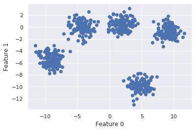
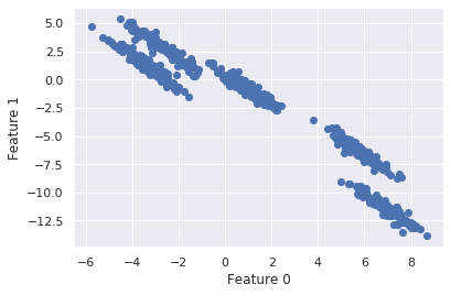
We have arguably 5 defined clusters with a stretched diagonal shape.

Let’s apply k-means clustering:

# cluster the data into five clusters
kmeans = KMeans(n_clusters=5)
kmeans.fit(X)
y_pred = kmeans.predict(X)# plot the cluster assignments and cluster centers
plt.scatter(X[:, 0], X[:, 1], c=y_pred, cmap="plasma")
plt.scatter(kmeans.cluster_centers_[:, 0],   
            kmeans.cluster_centers_[:, 1],
            marker='^', 
            c=[0, 1, 2, 3, 4], 
            s=100, 
            linewidth=2,
            cmap="plasma")plt.xlabel("Feature 0")
plt.ylabel("Feature 1")

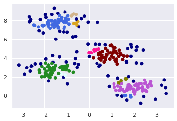
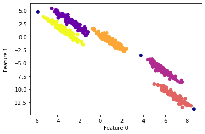
What we can see here is that k-means has been able to correctly detect the clusters at the middle and bottom, while presenting trouble with the clusters at the top, which are very close to each other. The Introduction to Machine Leaning with Python says “these groups are stretched toward the diagonal. As k-means only considers the distance to the nearest cluster center, it can’t handle this kind of data”.

DBSCAN

DBSCAN is an unsupervised machine learning algorithm to classify unlabeled data. DBSCAN is very weel suited for problems with:

1. Minimal domain knowledge to determine the input parameters (i.e. K in k-means and Dmin in hierarchical clustering)
2. Discovery of clusters with arbitrary shapes
3. Good efficiency on large databases

Find more in the original paper here.

Briefly, DBSCAN:

1. Stands for “density based spatial clustering of applications with noise”
2. Does not require the user to set the number of clusters a priori
3. Can capture clusters of complex shapes
4. Can identify points that are not part of any cluster (very useful as outliers detector)
5. Is somewhat slower than agglomerative clustering and k-means, but still scales to relatively large datasets
6. Works by identifying points that are in crowded regions of the feature space, where many data points are close together (dense regions in feature space)
7. Is very sensitive to scale since epsilon is a fixed value for the maximum distance between two points.

The Algorithm

Main parameters

1. eps ($epsilon$): Two points are considered neighbors if the distance between the two points is below the threshold epsilon.
2. min_samples: The minimum number of neighbors a given point should have in order to be classified as a core point. The point itself is included in the minimum number of samples.
3. metric: An additional parameter to use when calculating distance between instances in a feature array (i.e. euclidean distance)

The algorithm works by computing the distance between every point and all other points. We then place the points into one of three categories.

Terminology

Core point: A point with at least min_samples points whose distance with respect to the point is below the threshold defined by epsilon.

Border point: A point that isn’t in close proximity to at least min_samples points but is close enough to one or more core point. Border points are included in the cluster of the closest core point.

Noise point: Points that aren’t close enough to core points to be considered border points. Noise points are ignored. That is to say, they aren’t part of any cluster.

Implementation

Starting by importing the necessary modules:

import numpy as np
from sklearn.datasets.samples_generator import make_blobs
from sklearn.neighbors import NearestNeighbors
from sklearn.cluster import DBSCAN
from matplotlib import pyplot as plt
import seaborn as sns
sns.set()

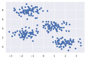
We will use the sklearn.datasets.make_blobs module to create the datam where we can see the clusters:

# make the dataset
X, y = make_blobs(n_samples=300, centers=4, cluster_std=0.60, random_state=0)
plt.scatter(X[:,0], X[:,1])
plt.show()

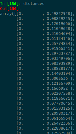
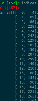
The next step is to find the right values for the min_sample and eps parameters, before running the DBSCAN. We can find a suitable value for epsilon by calculating the distance to the nearest n points for each point, sorting and plotting the results. Then we look to see where the change is most pronounced (think of the angle between your arm and forearm) and select that as epsilon. We can do that by using the sklearn.neighbors.NearestNeighbors. The kneighbors method returns two arrays, one which contains the distance to the closest n_neighbors points and the other which contains the index for each of those points.

# find the all distances between all points
neigh = NearestNeighbors(n_neighbors=2)
nbrs = neigh.fit(X)
distances, indices = nbrs.kneighbors(X)

Sorting and plotting the distances and:

# sort and plot the disctances to find the best eps parameters
distances = np.sort(distances, axis=0)
distances = distances[:,1]
plt.plot(distances)
plt.show()

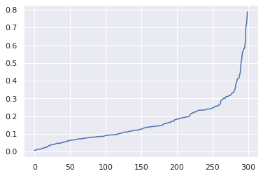
We see that the optimal eps (distance) is approximatelly 0.3. we can set min_samples to 5.

# run the DBSCAN algorithm
m = DBSCAN(eps=0.3, min_samples=5)
m.fit(X)

We can now see the clusters by running:

clusters = m.labels_

Mapping each cluster to a color using the numpy.vectorize module:

# map each cluster to a color and plot
colors = ['royalblue', 'maroon', 'forestgreen', 'mediumorchid', 'tan', 'deeppink', 'olive', 'goldenrod', 'lightcyan', 'navy']
vectorizer = np.vectorize(lambda x: colors[x % len(colors)])
plt.scatter(X[:, 0], X[:, 1], c=vectorizer(clusters))
plt.show()

The model classified the densely populated areas. The dark blue points were categorized as noise.

Second Implementation - kmeans and DBSCAN in the same dataset

Here we dive stright into the code:

import numpy as np
import matplotlib.pyplot as plt
from sklearn.datasets import make_blobs
from sklearn.cluster import KMeans, DBSCAN
from sklearn.preprocessing import StandardScaler
from sklearn.metrics.cluster import adjusted_rand_score

# make and plot dataset
X, y = make_blobs(random_state=170, n_samples=600, centers = 5)
plt.scatter(X[:, 0], X[:, 1])
plt.xlabel("Feature 0")
plt.ylabel("Feature 1")
plt.show()

# transform the data by stretching and plot
rng = np.random.RandomState(74)
transformation = rng.normal(size=(2, 2))
X = np.dot(X, transformation)
plt.scatter(X[:, 0], X[:, 1])
plt.xlabel("Feature 0")
plt.ylabel("Feature 1")
plt.show()

#apply k-means
kmeans = KMeans(n_clusters=5)
kmeans.fit(X)
y_pred = kmeans.predict(X)# plot the cluster assignments and cluster centers
plt.scatter(X[:, 0], X[:, 1], c=y_pred, cmap="plasma")
plt.scatter(kmeans.cluster_centers_[:, 0],   
            kmeans.cluster_centers_[:, 1],
            marker='^', 
            c=[0, 1, 2, 3, 4], 
            s=100, 
            linewidth=2,
            cmap="plasma")
plt.xlabel("Feature 0")
plt.ylabel("Feature 1")
plt.show()

#apply DBSCAN
scaler = StandardScaler()
X_scaled = scaler.fit_transform(X)# cluster the data into five clusters
dbscan = DBSCAN(eps=0.123, min_samples = 2)
clusters = dbscan.fit_predict(X_scaled)# plot the cluster assignments
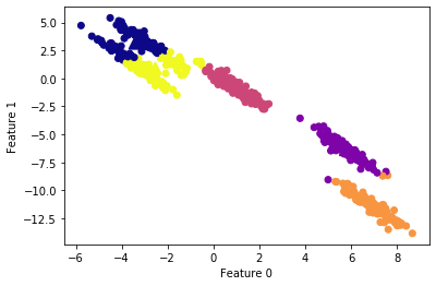
plt.scatter(X[:, 0], X[:, 1], c=clusters, cmap="plasma")
plt.xlabel("Feature 0")
plt.ylabel("Feature 1")
plt.show()

Important points

1. The parameter eps is somewhat more important, as it determines what it means for points to be close. Setting eps to be very small will mean that no points are core samples, and may lead to all points being labeled as noise. Setting eps to be very large will result in all points forming a single cluster.
2. While DBSCAN doesn’t require setting the number of clusters explicitly, setting eps implicitly controls how many clusters will be found.
3. Finding a good setting for eps is sometimes easier after scaling the data, as using these scaling techniques will ensure that all features have similar ranges.

Evaluation

We can measure the performance of our algorithms using adjusted_rand_score.

#k-means performance:
print("ARI =", adjusted_rand_score(y, y_pred).round(2))

ARI = 0.76

#DBSCAN performance:
print("ARI =", adjusted_rand_score(y, clusters).round(2))

ARI = 0.99

sources:

1. DBSCAN clustering for data shapes k-means can’t handle well by Gabriel Pierobon
2. DBSCAN Python Example: The Optimal Value For Epsilon (EPS) by Cory Maklin
3. Introduction to Machine Leaning with Python by Andreas C. Müller, Sarah Guido